Generalized Realtime Julia Set Fractals Using WebGL and Computer Algebra

Abstract

Background

Julia set fractals

In the first decades of the twentieth century, Pierre Fatou began investigating the dynamic properties of rational functions of polynomials on the unit disc when iterated repeatedly. Following his work, Gaston Julia looked into the properties of single-point trajectories of specific functions, including z = z^2 - 2. Today, the Fatou set refers to initial points whose trajectories converge, forming a closed set, while the Julia set refers to the initial points which diverge — especially on the boundaries of the Fatou set.

Julia set for c = -0.6078 + i*0.4380. Click to interact.

Mandelbrot set. Click to interact.

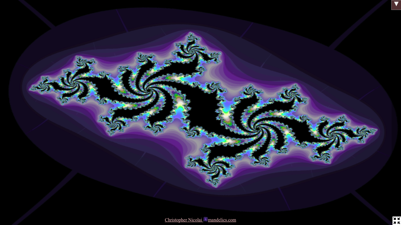
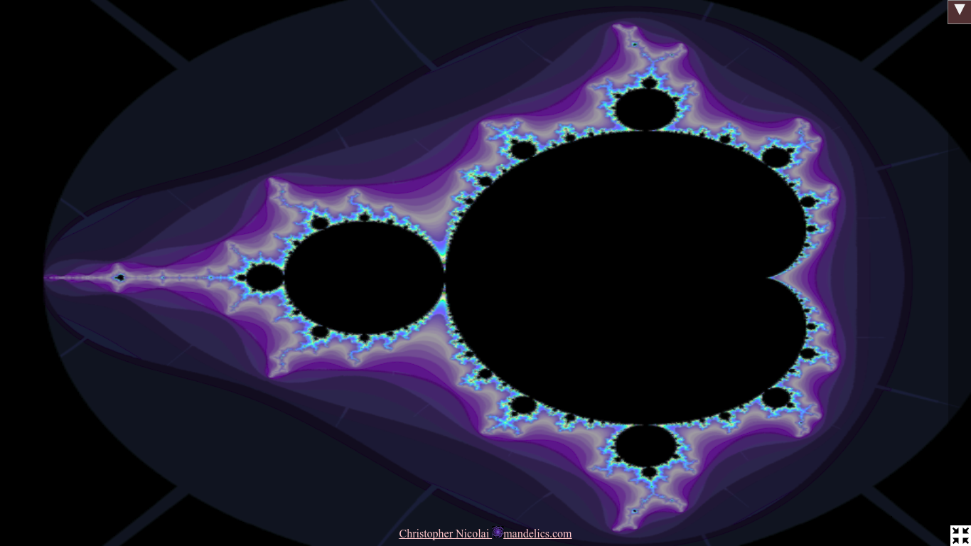
When computers became fast enough, Benoit Mandelbrot used them to visualize these dynamics. Mapping each pixel to an initial point z₀, he assigned to each a color based on how many iterations it took to escape a fixed disc. Mandelbrot introduced the set derived from z = z^2 + z₀, which bears his name.

For brevity, we will refer to all of the above as "Julia sets."

A member of the Mandelbrot set converges with a squarelike spiral trajectory.

Another trajectory near the set's boundary. Trajectories from outside the set (outside the black center) get larger instead of converging to a fixed point or attractor.

Julia computed his results by hand. In order to iterate his example, z = z^2 - 2, the complex variable z would have to be split into real and imaginary components:

Many programmers have worked under similar constraints — from classic C to modern WebGL, most environments have had limited support for complex math. Consequently, most visual explorations have focused on a limited quadratic family of sets. By automating the algebra, we aim to explore a broader family of Julia sets.

WebGL realtime fractals

WebGL is a widely available, cross-vendor, cross-platform standard for communicating with graphics cards (GPUs). It combines a "shader language" for programs which run on the GPU with an API to configure and invoke programs, accessed via JavaScript embedded in a web page. A shader program combines a "vertex shader" and a "fragment shader." The vertex shader is used to determine the onscreen position and relative depth of each vertex of a polygon, typically a triangle. The fragment shader is called on each visible point inside the polygon, to determine its color. Importantly for our approach, the shaders are compiled from text at runtime.

GPUs are more typically used for 3D scenes, which can have tens of thousands of triangles onscreen (plus more triangles rendered to offscreen textures for reflections, etc.), and require frame rates above 60 per second. A planar fractal needs only two triangles to make up a square. That leaves enough power to run several Julia iterations per pixel. In contrast to recent approaches using ping-pong buffers and enhanced floating point resolution, we compute all iterations in one pass at native GPU resolution.

In this paper, we'll use the WebGL term "uniform" for a run-time argument to a shader program. "Vector" will refer to WebGL's vec2 type, which has two single-precison float components. Vector addition is componentwise, but otherwise they do not behave like complex numbers. Thus, we need algebra to encode an otherwise-simple complex expression such as z = z^p + c, where p is provided at runtime as a uniform.

Implementation

To allow color animation and adjustable resolution, and to save processing time, we render in multiple stages. The primary shader program "draws" the numerical iteration count to an offscreen texture at the desired resolution. The secondary shader reads from that texture, and also writes to an offscreen texture, using the iteration number and animation time to pick a color from a "palette" texture. Finally, the color picture is scaled to fit the screen. The primary shader is only used when the coordinate system changes (e.g. pan and zoom), or when c changes. The user can adjust c dynamically by dragging along the display, or using the orientation (tilt) sensor available in most mobile browsers.

Our initial implementation, with z = z^2 + c expanded by hand, ran acceptably on a business-class laptop from 2011 with an integrated Intel HD Graphics 3000 GPU, achieving 29-59 frames per second (fps) at a resolution of 755x755 pixels. Some newer GPUs have over 280 times the processing power (by published GFLOPS benchmarks), suggesting it is tractable to visualize more complicated sets in real time.

Computer algebra systems

Computer algebra systems are programs which can manipulate symbolic mathematical expressions. They are commonly used to simplify expressions, for example by factoring, or to find analytical derivatives and integrals. We would like to expand any simple expression into its real and complex parts.

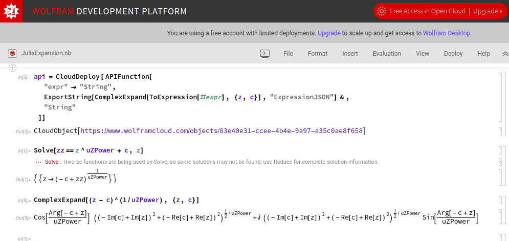
This can be accomplished with the Mathematica function ComplexExpand[]. For example, the input "ComplexExpand[z^p + c, {z,c}]" yields a general formula for any power p. We can transcribe this formula to WebGL, and animate p with a uniform. Surprisingly, Mathematica's built-in JuliaSetPlot[] function is limited to integer powers.

Mathematica is a classic computer algebra system, accessed using the dialect called "Wolfram Language" (WL). Like most computer algebra systems, it doesn't offer direct access to GPU APIs. Still, it's an appropriate choice here because of its long record of staying relevant, and because the Wolfram Cloud makes it easy to call WL functions over the internet via their Instant API service. The caller can even be from a non-WL environment, such as JavaScript/WebGL.

Generalized Julia set fractals using computer algebra

A:
varying and uniform declarations
polyfill atan2 definition
main function:
   initialize c from uniform
      if zero: c = z (mandelbrot)
   start iteration loop
B:
      z = f(z,c,uZPower)
C:
      break if escaped(z)
   output smoothed iteration count

The iteration function f(z) is just one part of the fragment shader, which also defines uniforms and helper functions, determines the pixel's z₀ coordinate, starts the iteration loop, tests after f(z) for escape (divergence), and records the iteration count. We implement the fragment shader as a template, lacking only z = f(z), which is generated from translated user input. The uniform uZPower is available, controlled by a slider. By default, we display f(z) = z^uZPower + c.

Complex expansion is accomplished using the Wolfram Cloud. We transform the expanded function with ExportString[..., "ExpressionJSON"], which generates a lisp-like representation of the WL syntax tree. For example, "a+(b*c)" is encoded as "["Add", "a", ["Plus", "b", "c"]]." This format is easily rewritten as WebGL shader code. A few notes:

Top: Publishing a Wolfram Cloud "Instant API" function. Argument and result have type String. The expanded expression is exported to ExpressionJSON, a lisp-like textual representation for the Wolfram Language. The ExportString function prevents newline and tab characters from being replaced with escape sequences.

Bottom: Expansion of (an) inverse function, z = (z - c)^(1/uZPower) in terms of real and imaginary source components.

• the complex components are output in the form "z = vec2({real},{imaginary});"
• ["Re", "c"] becomes c.x, and ["Im", "c"] becomes c.y;
• ["Arg", "c"] becomes atan2(c.y, c.x) (and atan2 must be defined in the template);
• integral numbers need a trailing dot in order to be interpreted as type float;
• most function names can simply be converted to lowercase, e.g. Sin becomes sin;
• ["Times", x, y] is handled specially, to separate the top-level real and imaginary components. If the first argument is ["Complex", 0, 1], the other argument is formatted separately as the imaginary component;
• there may be other WL functions that could occur; we handle all cases that occurred in our testing with ratios of polynomials.

Update: Computer Algebra with SAGE

After some time had passed, and I hadn't logged in to the free Wolfram Cloud account, it stopped working. Even if I kept maintaining it, there was a chance I'd have to start paying for the service. I found that SAGE, a Python-based mathematics suite, can also perform complex expansion.

I installed SAGE on the debian-based server: `sudo apt install sagemath`. The following script emulates the output from Wolfram Cloud:

# Reads a complex mathematical expression in SAGE notation from stdin, and writes its complex expansion to stdout,
# in the same form as Wolfram's `ExportString[ComplexExpand[ToExpression[#expr], {z, c}], "ExpressionJSON"]`.

import argparse
import builtins
import os
import sys
import sage.all

# We basically want SAGE syntax, but we'll also allow `^` for exponentiation
# Also prevent some meta-mischief a la `().__class__.__bases__[0].__subclasses__()[40]`
# (https://blog.osiris.cyber.nyu.edu/ctf/exploitation techniques/2012/10/26/escaping-python-sandboxes/)

def preprocess(input):
    return input.strip().replace('^', '**').replace('__', 'zz')

# Keeping WL names and capitalization for compatibility

class Remapping(dict):
    """Dict which returns the key itself if not found (to selectively rename things)."""
    def __getitem__(self, key):
        return key if not (key in self) else super(Remapping, self).__getitem__(key)

remap = Remapping({
    'Mul': 'Times',
    'Add': 'Plus',
    'Pow': 'Power',
    'Arctan2': 'Atan2',
    'Real': 'Re',
    'Imag': 'Im',
    'pi': 'Pi'
})

# The old solution exported the answer in Wolfram's ExpressionJSON format;
# basicaly S-expressions with the function and variable names as strings.

def quoted(x):
    return '"%s"' % x

def sage_to_name(x):
    return quoted(remap[ str(x) ])

# Some of SAGE's numbers are fractions or symbolic constants;

def sage_to_leaf(x):
    if x.is_numeric():
        if x.denominator() == 1: return str(x)
        else: return '["Rational", %s, %s]' % (x.numerator(), x.denominator())
    else:
        return sage_to_name(x)

# To transform SAGE function names into WL-style, we have to
# * find the name
# * strip the underscore and anything after (e.g. add_varargs)
# * capitalize
# * remap known differences

def sage_to_funcname(op):
    fn = op.name() if hasattr(op, 'name') else op.__name__
    if '_' in fn: fn = fn[:fn.index('_')]
    return sage_to_name(fn.capitalize())

# SAGE expressions can be traversed recursively via .operator() and .operands();
# we transform them into JSON-compatible S-expressions.

def sage_to_tree(expr):
    op = expr.operator()
    if op == None: return sage_to_leaf(expr)
    return '[' + ', '.join([sage_to_funcname(op)] + map(sage_to_tree, expr.operands())) + ']'

# Wolfram's ComplexExpand function returns an expression in the form f() + i * g(), still expected downstream.

def complex_expand(expr):
    real, imag = map(sage_to_tree, (expr.real(), expr.imag()))
    return """["Plus", %(real)s, ["Times", ["Complex", 0, 1], %(imag)s]]""" % locals()

# Since we accept arbitrary input online, we limit the available functions to just relevant math.

def build_global_vars():
    sage_globals = sage.all.__dict__
    builtin = builtins.__dict__
    allowed_globals = [
        'pi', 'I', 'e',
        'cos', 'sin', 'tan',
        'acos', 'asin', 'atan',
        'cosh', 'sinh', 'tanh',
        'acosh', 'asinh', 'atanh',
        'sqrt', 'exp', 'log',
        'pow', 'abs'
    ]
    expr_globals = dict([(name, sage_globals[name] if name in sage_globals else builtin[name]) for name in allowed_globals])
    expr_globals['__builtins__'] = {} # https://nedbatchelder.com/blog/201206/eval_really_is_dangerous.html
    return expr_globals

# We also limit the user to approved locals: all the desired complex and real SAGE vars.

def build_local_vars(v_complex=[], v_real=[]):
    return dict(
        [(v, sage.all.var(v)) for v in v_complex] +
        [(v, sage.all.var(v, domain='real')) for v in v_real]
    )

def parse_args():
    parser = argparse.ArgumentParser(description='Expand a complex expression into Wolfram-style JSON')
    parser.add_argument('--complex', default='z,c', help='list of complex variables allowed')
    parser.add_argument('--real', default='p,q,r', help='list of real variables allowed')
    return parser.parse_args()

def main():
    args = parse_args()
    expr_globals = build_global_vars()
    expr_locals = build_local_vars(args.complex.split(','), args.real.split(','))

    raw_expr = preprocess(sys.stdin.readline())
    expr = eval(raw_expr, expr_globals, expr_locals)
    
    if os.environ.has_key('DBG') and os.environ['DBG']:
        print("real: %s" % expr.real())
        print("imag: %s" % expr.imag())
    else:
        print(complex_expand(expr))

if __name__ == '__main__':
    main()
    

The expression is passed via stdin to avoid shell injection vulnerabilities. We `eval` with custom `globals` and `locals` to avoid python injection vulnerabilities. To guard against DOS via non-terminating expressions, the caller should impose a timeout.

Results

We have developed a program to visualize Julia sets of any user-provided f(z), combining GPU and computer algebra facilities not commonly found together. Functions and parameters can be changed in real time, enabling intuitive exploration of an expanded class of fractals. The program is available at https://mandelics.com/photo. For source code, press F12 while visiting the page.

Compiling and replacing two fragment shaders took less than 90 ms. Calling the Wolfram API took about 350 ms.

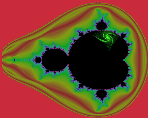
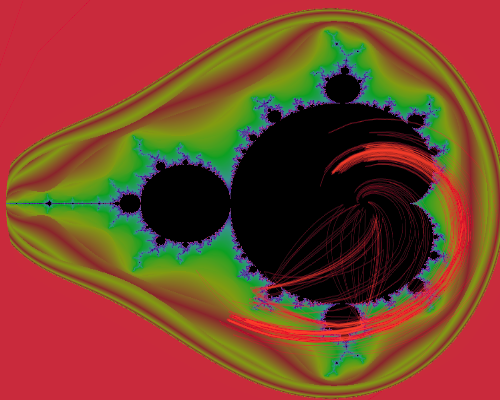
Using the general formula for z = z^p + c on a dated, business-class integrated GPU, we achieved frame rates that were generally above 30 per second; except on images where a large fraction of pixels never escape; Then, frame rates dropped as low as 2 per second.

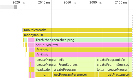
Switching the iteration function took less than half a second overall. It took about 350 ms to receive a response from the Wolfram Cloud, and an additional 90 ms to recompile and replace the shader programs. (Our program has two rendering modes; replacing a single mode would take only 60 ms.) Average frame rates stayed above 30 per second, except on highly convergent images. We produced rare new images of (an) inverse of the most famous Julia function, z = (z - c)^(1/uZPower).